GSP273

Overview
In this lab you create a Vertex AI Workbench instance on which you devlop a TensorFlow model in Jupyter notebook. You train the model, create an input data pipeline, deploy it to an endpoint, and get predictions.
TensorFlow is an end-to-end open source platform for machine learning. It has a comprehensive, flexible ecosystem of tools, libraries, and community resources that lets researchers push the state-of-the-art in ML and developers easily build and deploy ML powered applications.
Vertex AI brings AutoML and AI Platform together into a unified API, client library, and user interface. With Vertex AI, both AutoML training and custom training are available options.
Vertex AI Workbench helps users quickly build end-to-end notebook-based workflows through deep integration with data services (like Dataproc, Dataflow, BigQuery, and Dataplex) and Vertex AI. It enables data scientists to connect to Google Cloud data services, analyze datasets, experiment with different modeling techniques, deploy trained models into production, and manage MLOps through the model lifecycle.
Vertex AI Workbench is a single development environment for the entire data science workflow.
This lab uses a set of code samples and scripts developed for Data Science on the Google Cloud Platform, 2nd Edition from O'Reilly Media, Inc.
Objectives
- Deploy Vertex AI Workbench instance
- Create minimal training, validation data
- Create the input data pipeline
- Create TensorFlow model
- Deploy model to Vertex AI
- Deploy Explainable AI model to Vertex AI
- Make predictions from the model endpoint
Setup and requirements
Before you click the Start Lab button
Read these instructions. Labs are timed and you cannot pause them. The timer, which starts when you click Start Lab, shows how long Google Cloud resources will be made available to you.
This hands-on lab lets you do the lab activities yourself in a real cloud environment, not in a simulation or demo environment. It does so by giving you new, temporary credentials that you use to sign in and access Google Cloud for the duration of the lab.
To complete this lab, you need:
- Access to a standard internet browser (Chrome browser recommended).
Note: Use an Incognito or private browser window to run this lab. This prevents any conflicts between your personal account and the Student account, which may cause extra charges incurred to your personal account.
- Time to complete the lab---remember, once you start, you cannot pause a lab.
Note: If you already have your own personal Google Cloud account or project, do not use it for this lab to avoid extra charges to your account.
How to start your lab and sign in to the Google Cloud console
-
Click the Start Lab button. If you need to pay for the lab, a pop-up opens for you to select your payment method.
On the left is the Lab Details panel with the following:
- The Open Google Cloud console button
- Time remaining
- The temporary credentials that you must use for this lab
- Other information, if needed, to step through this lab
-
Click Open Google Cloud console (or right-click and select Open Link in Incognito Window if you are running the Chrome browser).
The lab spins up resources, and then opens another tab that shows the Sign in page.
Tip: Arrange the tabs in separate windows, side-by-side.
Note: If you see the Choose an account dialog, click Use Another Account.
-
If necessary, copy the Username below and paste it into the Sign in dialog.
{{{user_0.username | "Username"}}}
You can also find the Username in the Lab Details panel.
-
Click Next.
-
Copy the Password below and paste it into the Welcome dialog.
{{{user_0.password | "Password"}}}
You can also find the Password in the Lab Details panel.
-
Click Next.
Important: You must use the credentials the lab provides you. Do not use your Google Cloud account credentials.
Note: Using your own Google Cloud account for this lab may incur extra charges.
-
Click through the subsequent pages:
- Accept the terms and conditions.
- Do not add recovery options or two-factor authentication (because this is a temporary account).
- Do not sign up for free trials.
After a few moments, the Google Cloud console opens in this tab.
Note: To view a menu with a list of Google Cloud products and services, click the Navigation menu at the top-left.
Task 1. Deploy Vertex AI Workbench instance
-
In the Google Cloud Console, on the Navigation menu, click Vertex AI > Workbench.
-
Click + Create New.
-
In the Create instance dialog, use the default name or enter a unique name for the Vertex AI Workbench Instance. Set the region to and zone to and leave the rest of the settings as default.
-
Click Create.
-
Click Open JupyterLab.
To use a Notebook, you enter commands into a cell. Be sure you run the commands in the cell by either pressing Shift + Enter, or clicking the triangle on the Notebook top menu to Run selected cells and advance.
Deploy Vertex AI Workbench instance
Task 2. Create minimal training and validation data
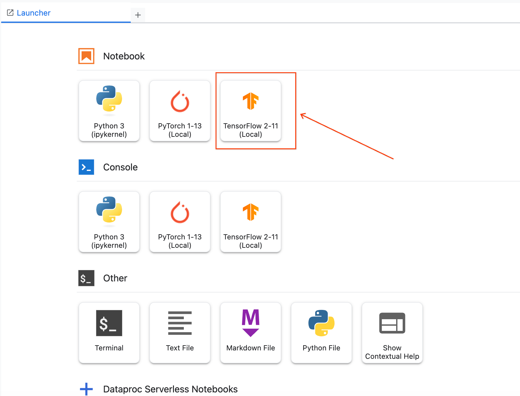
- In the Notebook launcher section click TensorFlow 2-11 (Local) to open a new notebook.
- Import Python libraries and set environment variables:
import os, json, math, shutil
import numpy as np
import tensorflow as tf
!sudo apt install graphviz -y
# environment variables used by bash cells
PROJECT=!(gcloud config get-value project)
PROJECT=PROJECT[0]
REGION = '{{{project_0.default_region}}}'
BUCKET='{}-dsongcp'.format(PROJECT)
os.environ['ENDPOINT_NAME'] = 'flights'
os.environ['BUCKET'] = BUCKET
os.environ['REGION'] = REGION
os.environ['TF_VERSION']='2-' + tf.__version__[2:4]
Note:
When pasting commands into the Jupyter notebook cell, remember to run the cell to be sure the last command in any sequence is executed before you proceed to the next step.
You can ignore any TensorRT Library Load or TensorFlow AVX2 FMA warnings.
Export files that contain training, validation data
When the lab spins up, a few tables are created in the BigQuery dataset. In this section, you use BigQuery to create temporary tables in BigQuery that contain the data we need, and then export the table to CSV files on Google Cloud Storage. You then delete the temporary table. Moving further, read and process those CSV data files to create the training, validation, and full datasets you need for a custom TensorFlow model.
- Create training dataset
flights_train_data for model training:
%%bigquery
CREATE OR REPLACE TABLE dsongcp.flights_train_data AS
SELECT
IF(arr_delay < 15, 1.0, 0.0) AS ontime,
dep_delay,
taxi_out,
distance,
origin,
dest,
EXTRACT(hour FROM dep_time) AS dep_hour,
IF (EXTRACT(dayofweek FROM dep_time) BETWEEN 2 AND 6, 1, 0) AS is_weekday,
UNIQUE_CARRIER AS carrier,
dep_airport_lat,
dep_airport_lon,
arr_airport_lat,
arr_airport_lon
FROM dsongcp.flights_tzcorr f
JOIN dsongcp.trainday t
ON f.FL_DATE = t.FL_DATE
WHERE
f.CANCELLED = False AND
f.DIVERTED = False AND
is_train_day = 'True'
- Create the evaluation dataset
flights_eval_data for model evaluation:
%%bigquery
CREATE OR REPLACE TABLE dsongcp.flights_eval_data AS
SELECT
IF(arr_delay < 15, 1.0, 0.0) AS ontime,
dep_delay,
taxi_out,
distance,
origin,
dest,
EXTRACT(hour FROM dep_time) AS dep_hour,
IF (EXTRACT(dayofweek FROM dep_time) BETWEEN 2 AND 6, 1, 0) AS is_weekday,
UNIQUE_CARRIER AS carrier,
dep_airport_lat,
dep_airport_lon,
arr_airport_lat,
arr_airport_lon
FROM dsongcp.flights_tzcorr f
JOIN dsongcp.trainday t
ON f.FL_DATE = t.FL_DATE
WHERE
f.CANCELLED = False AND
f.DIVERTED = False AND
is_train_day = 'False'
- Create the full dataset
flights_all_data using the following code:
%%bigquery
CREATE OR REPLACE TABLE dsongcp.flights_all_data AS
SELECT
IF(arr_delay < 15, 1.0, 0.0) AS ontime,
dep_delay,
taxi_out,
distance,
origin,
dest,
EXTRACT(hour FROM dep_time) AS dep_hour,
IF (EXTRACT(dayofweek FROM dep_time) BETWEEN 2 AND 6, 1, 0) AS is_weekday,
UNIQUE_CARRIER AS carrier,
dep_airport_lat,
dep_airport_lon,
arr_airport_lat,
arr_airport_lon,
IF (is_train_day = 'True',
IF(ABS(MOD(FARM_FINGERPRINT(CAST(f.FL_DATE AS STRING)), 100)) < 60, 'TRAIN', 'VALIDATE'),
'TEST') AS data_split
FROM dsongcp.flights_tzcorr f
JOIN dsongcp.trainday t
ON f.FL_DATE = t.FL_DATE
WHERE
f.CANCELLED = False AND
f.DIVERTED = False
- Export the training, validation, and full datasets to CSV file format the Google Cloud Storage bucket:
This will take about 2 minutes to complete.
- Wait until you receive output from running the following bash script in your notebook cell:
%%bash
PROJECT=$(gcloud config get-value project)
for dataset in "train" "eval" "all"; do
TABLE=dsongcp.flights_${dataset}_data
CSV=gs://${BUCKET}/ch9/data/${dataset}.csv
echo "Exporting ${TABLE} to ${CSV} and deleting table"
bq --project_id=${PROJECT} extract --destination_format=CSV $TABLE $CSV
bq --project_id=${PROJECT} rm -f $TABLE
done
- List exported objects to Google Cloud Storage bucket using the following code:
!gsutil ls -lh gs://{BUCKET}/ch9/data
Create training and validation dataset
Task 3. Create the input data
Setup in notebook
- For development purposes, train for a few epochs. That's why the NUM_EXAMPLES is so low.
DEVELOP_MODE = True
NUM_EXAMPLES = 5000*1000
- Assign your training and validation data URI to
training_data_uri and validation_data_uri respectively:
training_data_uri = 'gs://{}/ch9/data/train*'.format(BUCKET)
validation_data_uri = 'gs://{}/ch9/data/eval*'.format(BUCKET)
- Set up Model Parameters using the following code-block:
NBUCKETS = 5
NEMBEDS = 3
TRAIN_BATCH_SIZE = 64
DNN_HIDDEN_UNITS = '64,32'
Reading data into TensorFlow
- To read the CSV files from Google Cloud Storage into TensorFlow, use a method from the
tf.data package:
if DEVELOP_MODE:
train_df = tf.data.experimental.make_csv_dataset(training_data_uri, batch_size=5)
for n, data in enumerate(train_df):
numpy_data = {k: v.numpy() for k, v in data.items()}
print(n, numpy_data)
if n==1: break
Write features_and_labels() and read_dataset() functions. The read_dataset() function reads the training data, yielding batch_size examples each time, and allows you to stop iterating once a certain number of examples have been read.
The dataset contains all the columns in the CSV file, named according to the header line. The data consists of both features and the label. It’s better to separate them by writing the features_and_labels() function to make the later code easier to read. Hence, we’ll apply a pop() function to the dictionary and return a tuple of features and labels).
- Enter and run the following code:
def features_and_labels(features):
label = features.pop('ontime')
return features, label
def read_dataset(pattern, batch_size, mode=tf.estimator.ModeKeys.TRAIN, truncate=None):
dataset = tf.data.experimental.make_csv_dataset(pattern, batch_size, num_epochs=1)
dataset = dataset.map(features_and_labels)
if mode == tf.estimator.ModeKeys.TRAIN:
dataset = dataset.shuffle(batch_size*10)
dataset = dataset.repeat()
dataset = dataset.prefetch(1)
if truncate is not None:
dataset = dataset.take(truncate)
return dataset
if DEVELOP_MODE:
print("Checking input pipeline")
one_item = read_dataset(training_data_uri, batch_size=2, truncate=1)
print(list(one_item)) # should print one batch of 2 items
Task 4. Create, train and evaluate TensorFlow model
Typically you create one feature for every column in our tabular data. Keras supports feature columns, opening up the ability to represent structured data using standard feature engineering techniques like embedding, bucketizing, and feature crosses.
As numeric data can be passed in directly to the ML model, keep the real-valued columns separate from the sparse (or string) columns:
- Enter and run the following code:
import tensorflow as tf
real = {
colname : tf.feature_column.numeric_column(colname)
for colname in
(
'dep_delay,taxi_out,distance,dep_hour,is_weekday,' +
'dep_airport_lat,dep_airport_lon,' +
'arr_airport_lat,arr_airport_lon'
).split(',')
}
sparse = {
'carrier': tf.feature_column.categorical_column_with_vocabulary_list('carrier',
vocabulary_list='AS,VX,F9,UA,US,WN,HA,EV,MQ,DL,OO,B6,NK,AA'.split(',')),
'origin' : tf.feature_column.categorical_column_with_hash_bucket('origin', hash_bucket_size=1000),
'dest' : tf.feature_column.categorical_column_with_hash_bucket('dest', hash_bucket_size=1000),
}
All these features come directly from the input file (and are provided by any client that wants a prediction for a flight). Input layers map 1:1 to the input features and their types, so rather than repeat the column names, you create an input layer for each of these columns, specifying the right data type (either a float or a string).
- Enter and run the following code:
inputs = {
colname : tf.keras.layers.Input(name=colname, shape=(), dtype='float32')
for colname in real.keys()
}
inputs.update({
colname : tf.keras.layers.Input(name=colname, shape=(), dtype='string')
for colname in sparse.keys()
})
Bucketing
Real-valued columns whose precision is overkill (thus, likely to cause overfitting) can be discretized and made into categorical columns. For example, if you have a column for the age of the aircraft, you might discretize into just three bins—less than 5 years old, 5 to 20 years old, and more than 20 years old. Use the discretization shortcut: you can discretize the latitudes and longitudes and cross the buckets—this results in breaking up the country into grids and yield the grid point into which a specific latitude and longitude falls.
- Enter and run the following code:
latbuckets = np.linspace(20.0, 50.0, NBUCKETS).tolist() # USA
lonbuckets = np.linspace(-120.0, -70.0, NBUCKETS).tolist() # USA
disc = {}
disc.update({
'd_{}'.format(key) : tf.feature_column.bucketized_column(real[key], latbuckets)
for key in ['dep_airport_lat', 'arr_airport_lat']
})
disc.update({
'd_{}'.format(key) : tf.feature_column.bucketized_column(real[key], lonbuckets)
for key in ['dep_airport_lon', 'arr_airport_lon']
})
# cross columns that make sense in combination
sparse['dep_loc'] = tf.feature_column.crossed_column(
[disc['d_dep_airport_lat'], disc['d_dep_airport_lon']], NBUCKETS*NBUCKETS)
sparse['arr_loc'] = tf.feature_column.crossed_column(
[disc['d_arr_airport_lat'], disc['d_arr_airport_lon']], NBUCKETS*NBUCKETS)
sparse['dep_arr'] = tf.feature_column.crossed_column([sparse['dep_loc'], sparse['arr_loc']], NBUCKETS ** 4)
# embed all the sparse columns
embed = {
'embed_{}'.format(colname) : tf.feature_column.embedding_column(col, NEMBEDS)
for colname, col in sparse.items()
}
real.update(embed)
# one-hot encode the sparse columns
sparse = {
colname : tf.feature_column.indicator_column(col)
for colname, col in sparse.items()
}
if DEVELOP_MODE:
print(sparse.keys())
print(real.keys())
Train and evaluate the model
- Save the checkpoint:
output_dir='gs://{}/ch9/trained_model'.format(BUCKET)
os.environ['OUTDIR'] = output_dir # needed for deployment
print('Writing trained model to {}'.format(output_dir))
- Delete the model checkpoints already present in the storage bucket:
!gsutil -m rm -rf $OUTDIR
This reports an error stating CommandException: 1 files/objects could not be removed because the model has not yet been saved. The error indicates that there are no files present in the target location. You must be certain that this location is empty before attempting to save the model and this command guarantees that.
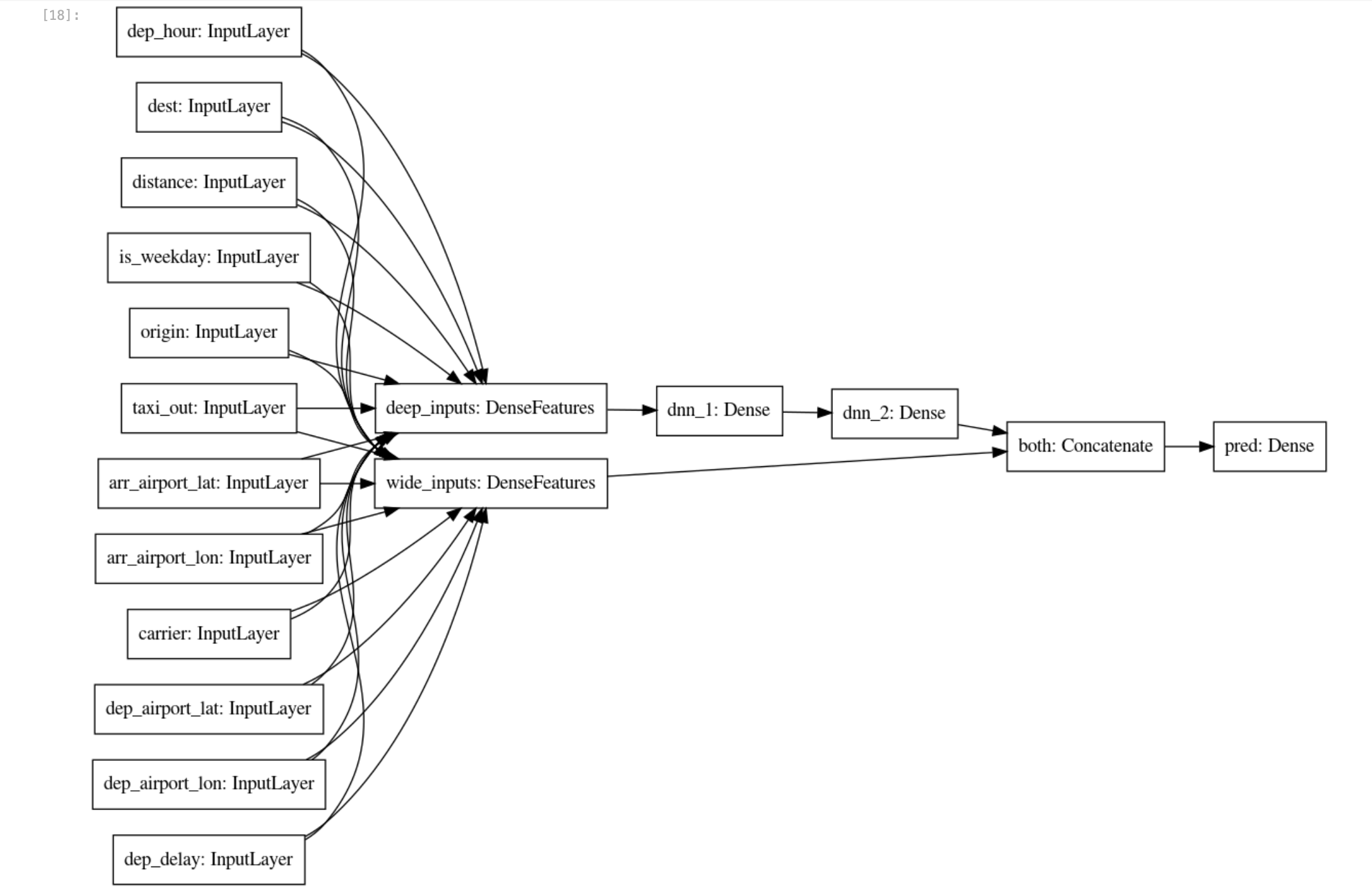
- With the sparse and real feature columns thus enhanced beyond the raw inputs, you can create a
wide_and_deep_classifier passing in the linear and deep feature columns separately:
# Build a wide-and-deep model.
def wide_and_deep_classifier(inputs, linear_feature_columns, dnn_feature_columns, dnn_hidden_units):
deep = tf.keras.layers.DenseFeatures(dnn_feature_columns, name='deep_inputs')(inputs)
layers = [int(x) for x in dnn_hidden_units.split(',')]
for layerno, numnodes in enumerate(layers):
deep = tf.keras.layers.Dense(numnodes, activation='relu', name='dnn_{}'.format(layerno+1))(deep)
wide = tf.keras.layers.DenseFeatures(linear_feature_columns, name='wide_inputs')(inputs)
both = tf.keras.layers.concatenate([deep, wide], name='both')
output = tf.keras.layers.Dense(1, activation='sigmoid', name='pred')(both)
model = tf.keras.Model(inputs, output)
model.compile(optimizer='adam',
loss='binary_crossentropy',
metrics=['accuracy'])
return model
model = wide_and_deep_classifier(
inputs,
linear_feature_columns = sparse.values(),
dnn_feature_columns = real.values(),
dnn_hidden_units = DNN_HIDDEN_UNITS)
tf.keras.utils.plot_model(model, 'flights_model.png', show_shapes=False, rankdir='LR')
Use train_dataset for model training and eval_dataset for model evaluation.
- Create the model using the following code-blocks:
# training and evaluation dataset
train_batch_size = TRAIN_BATCH_SIZE
if DEVELOP_MODE:
eval_batch_size = 100
steps_per_epoch = 3
epochs = 2
num_eval_examples = eval_batch_size*10
else:
eval_batch_size = 100
steps_per_epoch = NUM_EXAMPLES // train_batch_size
epochs = 10
num_eval_examples = eval_batch_size * 100
train_dataset = read_dataset(training_data_uri, train_batch_size)
eval_dataset = read_dataset(validation_data_uri, eval_batch_size, tf.estimator.ModeKeys.EVAL, num_eval_examples)
checkpoint_path = '{}/checkpoints/flights.cpt'.format(output_dir)
shutil.rmtree(checkpoint_path, ignore_errors=True)
cp_callback = tf.keras.callbacks.ModelCheckpoint(checkpoint_path,
save_weights_only=True,
verbose=1)
history = model.fit(train_dataset,
validation_data=eval_dataset,
epochs=epochs,
steps_per_epoch=steps_per_epoch,
callbacks=[cp_callback])
- Visualize the model loss and model accuracy using
matplotlib.pyplot:
import matplotlib.pyplot as plt
nrows = 1
ncols = 2
fig = plt.figure(figsize=(10, 5))
for idx, key in enumerate(['loss', 'accuracy']):
ax = fig.add_subplot(nrows, ncols, idx+1)
plt.plot(history.history[key])
plt.plot(history.history['val_{}'.format(key)])
plt.title('model {}'.format(key))
plt.ylabel(key)
plt.xlabel('epoch')
plt.legend(['train', 'validation'], loc='upper left');
The output looks similar to the following:
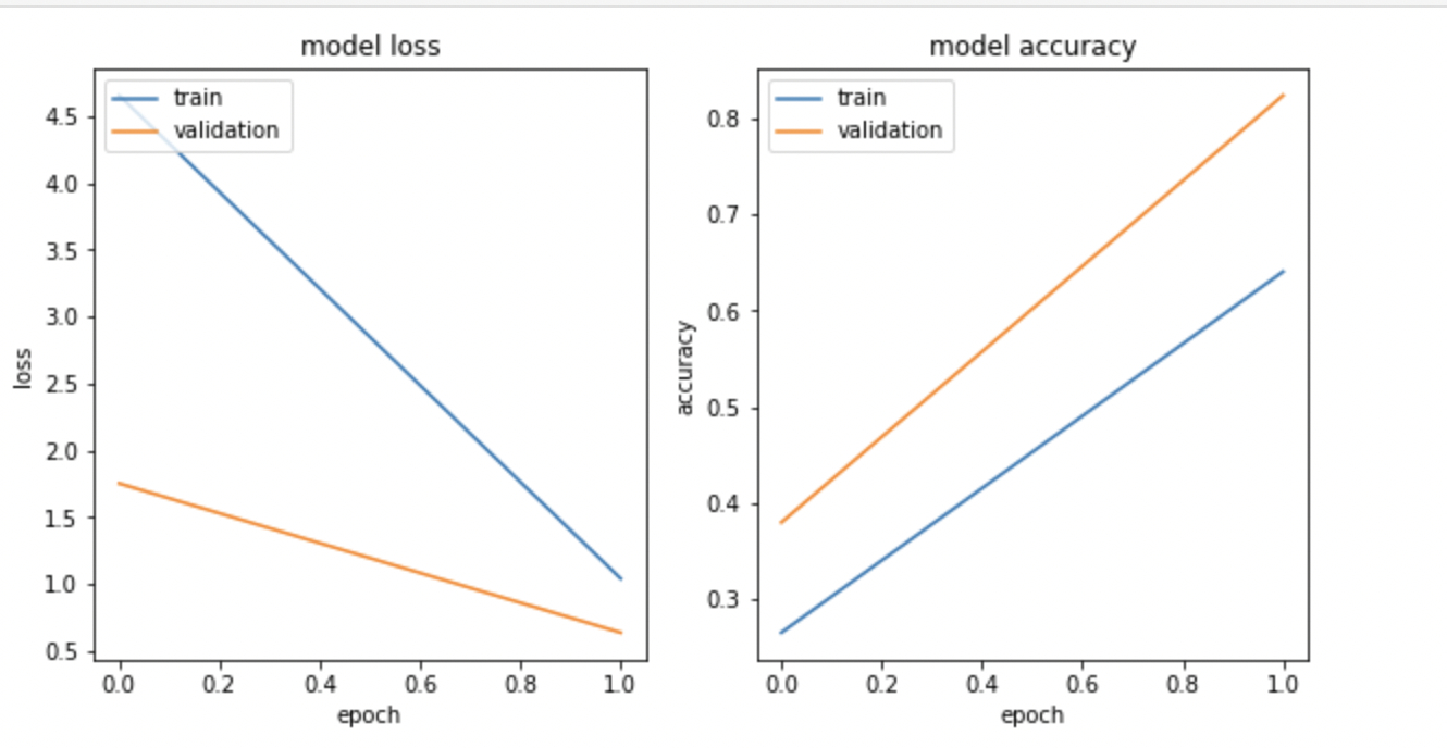
Note: Training loss and the model accuracy graph may not match because you are training on a very small random sample.
Export the trained model
- Save the model artifacts to the Google Cloud Storage bucket:
import time
export_dir = '{}/export/flights_{}'.format(output_dir, time.strftime("%Y%m%d-%H%M%S"))
print('Exporting to {}'.format(export_dir))
tf.saved_model.save(model, export_dir)
Create the TensorFlow Model
Task 5. Deploy flights model to Vertex AI
Vertex AI provides a fully managed, autoscaling, serverless environment for Machine Learning models. You get the benefits of paying for any compute resources (such as CPUs or GPUs) only when you are using them. Because the models are containerized, dependency management is taken care of. The Endpoints take care of traffic splits, allowing you to do A/B testing in a convenient way.
The benefits go beyond not having to manage infrastructure. Once you deploy the model to Vertex AI, you get a lot of neat capabilities without any additional code — explainability, drift detection, monitoring, etc.
- Create the model endpoint
flights using the following code cell and delete any existing models with the same name:
%%bash
# note TF_VERSION and ENDPOINT_NAME set in 1st cell
# TF_VERSION=2-6
# ENDPOINT_NAME=flights
TIMESTAMP=$(date +%Y%m%d-%H%M%S)
MODEL_NAME=${ENDPOINT_NAME}-${TIMESTAMP}
EXPORT_PATH=$(gsutil ls ${OUTDIR}/export | tail -1)
echo $EXPORT_PATH
# create the model endpoint for deploying the model
if [[ $(gcloud ai endpoints list --region=$REGION \
--format='value(DISPLAY_NAME)' --filter=display_name=${ENDPOINT_NAME}) ]]; then
echo "Endpoint for $MODEL_NAME already exists"
else
echo "Creating Endpoint for $MODEL_NAME"
gcloud ai endpoints create --region=${REGION} --display-name=${ENDPOINT_NAME}
fi
ENDPOINT_ID=$(gcloud ai endpoints list --region=$REGION \
--format='value(ENDPOINT_ID)' --filter=display_name=${ENDPOINT_NAME})
echo "ENDPOINT_ID=$ENDPOINT_ID"
# delete any existing models with this name
for MODEL_ID in $(gcloud ai models list --region=$REGION --format='value(MODEL_ID)' --filter=display_name=${MODEL_NAME}); do
echo "Deleting existing $MODEL_NAME ... $MODEL_ID "
gcloud ai models delete --region=$REGION $MODEL_ID
done
# create the model using the parameters docker conatiner image and artifact uri
gcloud ai models upload --region=$REGION --display-name=$MODEL_NAME \
--container-image-uri=us-docker.pkg.dev/vertex-ai/prediction/tf2-cpu.${TF_VERSION}:latest \
--artifact-uri=$EXPORT_PATH
MODEL_ID=$(gcloud ai models list --region=$REGION --format='value(MODEL_ID)' --filter=display_name=${MODEL_NAME})
echo "MODEL_ID=$MODEL_ID"
# deploy the model to the endpoint
gcloud ai endpoints deploy-model $ENDPOINT_ID \
--region=$REGION \
--model=$MODEL_ID \
--display-name=$MODEL_NAME \
--machine-type=e2-standard-2 \
--min-replica-count=1 \
--max-replica-count=1 \
--traffic-split=0=100
Note: An error can occasionally occur around 5 minutes into this process. If you encounter a model building error, like the service account doesn't have sufficient permissions for writing objects to the Google Cloud Storage bucket, try to run the code cell again. Also, enable the Vertex AI API, if not enabled.
Note: It will take around 15-20 minutes to create the model, model endpoint, and deploy the model to the endpoint. If you are unable to access the generated endpoint link, please ignore it. To see the progress in your Cloud Console, click on Navigation menu > Vertex AI > Online prediction > Endpoints.
Deploy flights model to Vertex AI
- Create a test input file
example_input.json using the following code:
%%writefile example_input.json
{"instances": [
{"dep_hour": 2, "is_weekday": 1, "dep_delay": 40, "taxi_out": 17, "distance": 41, "carrier": "AS", "dep_airport_lat": 58.42527778, "dep_airport_lon": -135.7075, "arr_airport_lat": 58.35472222, "arr_airport_lon": -134.57472222, "origin": "GST", "dest": "JNU"},
{"dep_hour": 22, "is_weekday": 0, "dep_delay": -7, "taxi_out": 7, "distance": 201, "carrier": "HA", "dep_airport_lat": 21.97611111, "dep_airport_lon": -159.33888889, "arr_airport_lat": 20.89861111, "arr_airport_lon": -156.43055556, "origin": "LIH", "dest": "OGG"}
]}
- Make a prediction from the model endpoint. Here you have input data in a JSON file called
example_input.json:
%%bash
ENDPOINT_ID=$(gcloud ai endpoints list --region=$REGION \
--format='value(ENDPOINT_ID)' --filter=display_name=${ENDPOINT_NAME})
echo $ENDPOINT_ID
gcloud ai endpoints predict $ENDPOINT_ID --region=$REGION --json-request=example_input.json
Here’s how client programs can invoke the model that you deployed.
Assume that they have the input data in a JSON file called example_input.json.
- Now, send an HTTP POST request and you will get the result back as JSON:
%%bash
PROJECT=$(gcloud config get-value project)
ENDPOINT_ID=$(gcloud ai endpoints list --region=$REGION \
--format='value(ENDPOINT_ID)' --filter=display_name=${ENDPOINT_NAME})
curl -X POST \
-H "Authorization: Bearer "$(gcloud auth application-default print-access-token) \
-H "Content-Type: application/json; charset=utf-8" \
-d @example_input.json \
"https://${REGION}-aiplatform.googleapis.com/v1/projects/${PROJECT}/locations/${REGION}/endpoints/${ENDPOINT_ID}:predict"
Task 6. Model explainability
Model explainability is one of the most important problems in machine learning. It's a broad concept of analyzing and understanding the results provided by machine learning models. Explainability in machine learning means you can explain what happens in your model from input to output. It makes models transparent and solves the black box problem. Explainable AI (XAI) is the more formal way to describe this.
- Run the following code:
%%bash
model_dir=$(gsutil ls ${OUTDIR}/export | tail -1)
echo $model_dir
saved_model_cli show --tag_set serve --signature_def serving_default --dir $model_dir
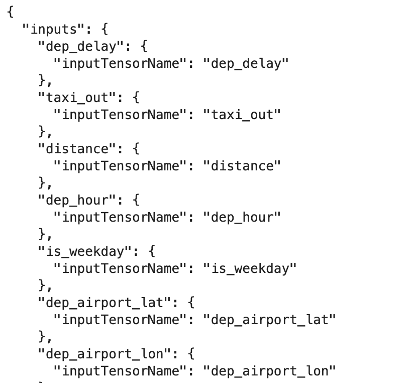
- Create a JSON file
explanation-metadata.json that contains the metadata describing the Model's input and output for explanation. Here, you use sampled-shapley method used for explanation:
cols = ('dep_delay,taxi_out,distance,dep_hour,is_weekday,' +
'dep_airport_lat,dep_airport_lon,' +
'arr_airport_lat,arr_airport_lon,' +
'carrier,origin,dest')
inputs = {x: {"inputTensorName": "{}".format(x)}
for x in cols.split(',')}
expl = {
"inputs": inputs,
"outputs": {
"pred": {
"outputTensorName": "pred"
}
}
}
print(expl)
with open('explanation-metadata.json', 'w') as ofp:
json.dump(expl, ofp, indent=2)
- View the
explanation-metadata.json file using the cat command:
!cat explanation-metadata.json
Create and deploy another model flights_xai to Vertex AI
- Create the model endpoint
flights_xai, upload the model, and deploy it at the model endpoint using the following code:
%%bash
# note ENDPOINT_NAME is being changed
ENDPOINT_NAME=flights_xai
TIMESTAMP=$(date +%Y%m%d-%H%M%S)
MODEL_NAME=${ENDPOINT_NAME}-${TIMESTAMP}
EXPORT_PATH=$(gsutil ls ${OUTDIR}/export | tail -1)
echo $EXPORT_PATH
# create the model endpoint for deploying the model
if [[ $(gcloud ai endpoints list --region=$REGION \
--format='value(DISPLAY_NAME)' --filter=display_name=${ENDPOINT_NAME}) ]]; then
echo "Endpoint for $MODEL_NAME already exists"
else
# create model endpoint
echo "Creating Endpoint for $MODEL_NAME"
gcloud ai endpoints create --region=${REGION} --display-name=${ENDPOINT_NAME}
fi
ENDPOINT_ID=$(gcloud ai endpoints list --region=$REGION \
--format='value(ENDPOINT_ID)' --filter=display_name=${ENDPOINT_NAME})
echo "ENDPOINT_ID=$ENDPOINT_ID"
# delete any existing models with this name
for MODEL_ID in $(gcloud ai models list --region=$REGION --format='value(MODEL_ID)' --filter=display_name=${MODEL_NAME}); do
echo "Deleting existing $MODEL_NAME ... $MODEL_ID "
gcloud ai models delete --region=$REGION $MODEL_ID
done
# upload the model using the parameters docker conatiner image, artifact URI, explanation method,
# explanation path count and explanation metadata JSON file `explanation-metadata.json`.
# Here, you keep number of feature permutations to `10` when approximating the Shapley values for explanation.
gcloud ai models upload --region=$REGION --display-name=$MODEL_NAME \
--container-image-uri=us-docker.pkg.dev/vertex-ai/prediction/tf2-cpu.${TF_VERSION}:latest \
--artifact-uri=$EXPORT_PATH \
--explanation-method=sampled-shapley --explanation-path-count=10 --explanation-metadata-file=explanation-metadata.json
MODEL_ID=$(gcloud ai models list --region=$REGION --format='value(MODEL_ID)' --filter=display_name=${MODEL_NAME})
echo "MODEL_ID=$MODEL_ID"
# deploy the model to the endpoint
gcloud ai endpoints deploy-model $ENDPOINT_ID \
--region=$REGION \
--model=$MODEL_ID \
--display-name=$MODEL_NAME \
--machine-type=e2-standard-2 \
--min-replica-count=1 \
--max-replica-count=1 \
--traffic-split=0=100
Note: It will take around 15-20 minutes to create the model, model endpoint, and deploy the model to the endpoint. If you are unable to access the generated endpoint link, please ignore it. To see the progress in your Cloud Console, click on Navigation menu > Vertex AI > Online prediction > Endpoints.
Deploy flights_xai model to Vertex AI
Task 7. Invoke the deployed model
Here’s how client programs can invoke the model you deployed. Assume that they have the input data in a JSON file called example_input.json. Now, send an HTTP POST request and you will get the result back as JSON.
%%bash
PROJECT=$(gcloud config get-value project)
ENDPOINT_NAME=flights_xai
ENDPOINT_ID=$(gcloud ai endpoints list --region=$REGION \
--format='value(ENDPOINT_ID)' --filter=display_name=${ENDPOINT_NAME})
curl -X POST \
-H "Authorization: Bearer "$(gcloud auth application-default print-access-token) \
-H "Content-Type: application/json; charset=utf-8" \
-d @example_input.json \
"https://${REGION}-aiplatform.googleapis.com/v1/projects/${PROJECT}/locations/${REGION}/endpoints/${ENDPOINT_ID}:explain"
Congratulations!
Congratulations! In this lab, you learned how to create a model using Vertex AI and deploy it to Vertex AI Endpoints. You also learned how to use the Vertex AI Explainable AI (XAI) feature to explain the model predictions. You then trained a logistic regression model on all of the input values and learned that the model was unable to effectively use the new features like airport locations.
Next Steps / Learn more
Google Cloud training and certification
...helps you make the most of Google Cloud technologies. Our classes include technical skills and best practices to help you get up to speed quickly and continue your learning journey. We offer fundamental to advanced level training, with on-demand, live, and virtual options to suit your busy schedule. Certifications help you validate and prove your skill and expertise in Google Cloud technologies.
Manual Last Updated December 28, 2023
Lab Last Tested December 28, 2023
Copyright 2024 Google LLC All rights reserved. Google and the Google logo are trademarks of Google LLC. All other company and product names may be trademarks of the respective companies with which they are associated.