Checkpoints
Check BigQuery datasets creation
/ 5
Check BigQuery tables creation
/ 5
Create a partioned table
/ 10
Check denormalized table creation
/ 10
Check cluster by order_id creation
/ 5
Check cluster by product_id creation
/ 5
Create a materialized view
/ 10
Create a table partition by order_ts
/ 5
Performance and Cost Optimization with BigQuery
- GSP266
- Overview
- Objectives
- Setup and requirements
- Importing data into your project
- Task 1: Create BigQuery tables and load data into the tables
- Task 2: Write SQL queries
- Task 3: Reduce the cost by making use of partitioning
- Task 4: Optimize a query by using denormalization
- Task 5: Improve row filtering and join performance by using clustering
- Task 6: Improve dashboard loading speed and cost by using materialized view
- Task 7: Reduce the elapsed time and cost by pruning partition with a filter
- Congratulations
GSP266

Overview
BigQuery is Google's fully managed, NoOps, low cost analytics database. With BigQuery you can query terabytes and terabytes of data without having any infrastructure to manage or needing a database administrator. BigQuery uses SQL and can take advantage of the pay-as-you-go model. BigQuery allows you to focus on analyzing data to find meaningful insights.
In this lab, you will learn to improve your database from a performance and cost perspective.
Objectives
In this lab, you will learn to:
- Create BigQuery tables and load data into it.
- Reduce the cost of a query by using partitioning.
- Optimize a query by using denormalization.
- Improve row filtering and join performance by using clustering.
- Improve dashboard loading speed and cost by using materialized view.
- Reduce the elapsed time and cost by pruning the partitions with filters.
- Save cost by moving data out of unused partitions in BigQuery and onto cheaper Google Cloud Storage.
Setup and requirements
Before you click the Start Lab button
Read these instructions. Labs are timed and you cannot pause them. The timer, which starts when you click Start Lab, shows how long Google Cloud resources will be made available to you.
This Qwiklabs hands-on lab lets you do the lab activities yourself in a real cloud environment, not in a simulation or demo environment. It does so by giving you new, temporary credentials that you use to sign in and access Google Cloud for the duration of the lab.
What you need
To complete this lab, you need:
- Access to a standard internet browser (Chrome browser recommended)
- Time to complete the lab
How to start your lab and sign in to the Google Cloud console
-
Click the Start Lab button. If you need to pay for the lab, a pop-up opens for you to select your payment method. On the left is the Lab details pane, which is populated with the temporary credentials that are needed for this lab.
-
Copy the Password and then click Open Google Cloud console. The lab spins up resources, then opens another tab that shows the Sign in page.
Tip: Open the tabs in separate windows, side by side. Note: If you see the Choose an account page, click Use another account. -
On the Sign in page, verify that the username from the Lab details pane is auto-filled. Click Next.
-
Paste the password in the Enter your password field. Click Next.
Important: Use the credentials from the Lab details pane. Using your personal Google Cloud account may incur charges to your account. -
Click through the subsequent pages:
-
Understand your account management.
-
Accept the terms and conditions.
-

After a few moments, the console opens.

Activate Cloud Shell
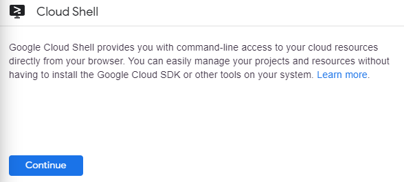
Cloud Shell is a virtual machine (VM) that is loaded with development tools. It offers a persistent 5GB home directory and runs on the Google Cloud. Cloud Shell provides command-line access to your Google Cloud resources.
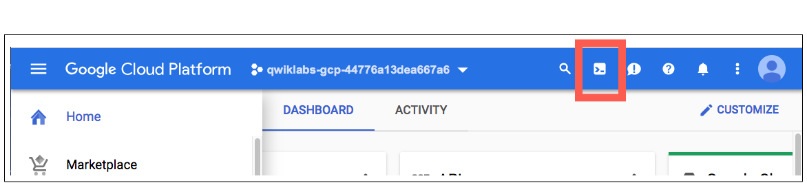
- In the Cloud Console, in the top-right toolbar, click the Activate Cloud Shell button.
- Click Continue.
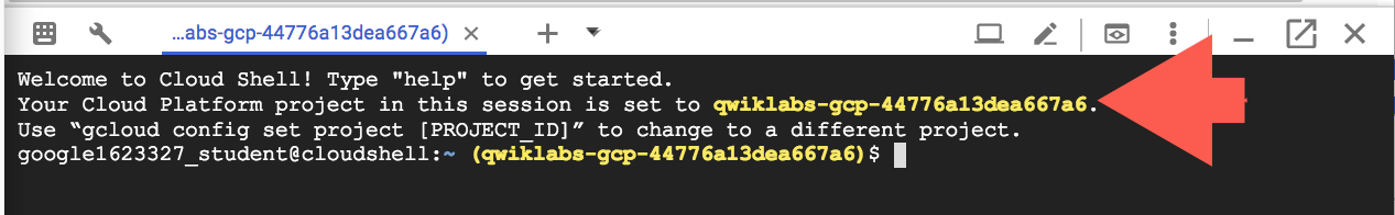
It takes a few moments to provision and connect to the environment. When you are connected, you are already authenticated, and the project is set to your PROJECT_ID. For example:
gcloud is the command-line tool for Google Cloud. It comes pre-installed on Cloud Shell and supports tab-completion.
- You can list the active account name with this command:
Output:
Example output:
- You can list the project ID with this command:
Output:
Example output:
gcloud see the gcloud command-line tool overview.
Importing data into your project
Now you will add an Instacart data warehouse data files into your Google Cloud project. This export is publicly available on Kaggle. To avoid creating a Kaggle account, the csv files have been uploaded to a publicly accessible Google Cloud Storage bucket for use with this lab.
- Execute the following to create an environment variable for your Google Cloud Project ID:
- Enter the following snippet into the command-line prompt to create a new bucket:
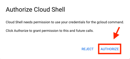
-
Click Authorize in the Authorize Cloud Shell dialog box that pops up.
-
Enter the following snippets into the command-line prompt to copy the Instacart data into your new bucket:
- Now confirm that all five CSV files have been uploaded to the bucket in your project:
- To lay the groundwork for this lab, three BigQuery datasets need to be created using the following commands:
Check BigQuery Datasets creation
Task 1: Create BigQuery tables and load data into the tables
- In Cloud Shell, run the following commands to create five tables and load data into these tables:
Check BigQuery tables creation
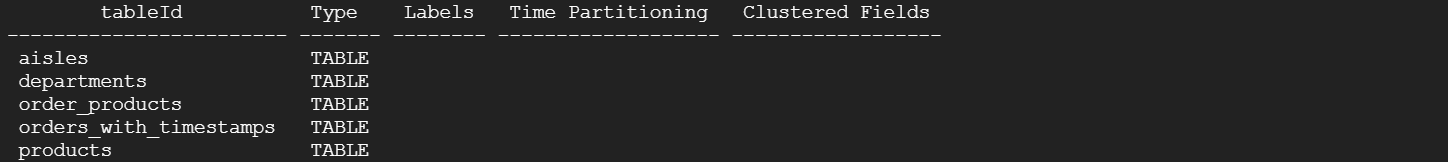
- Once those commands have finished, execute the following command to check that all five tables were created:
The output should be a table with contents similar to the output below:
Task 2: Write SQL queries
Below are a few questions regarding the data that you loaded into BigQuery tables earlier. Write SQL queries to solve the following problem statements in the BigQuery Editor and answer the questions. Also, note the bytes billed from the job details page for each of those queries.
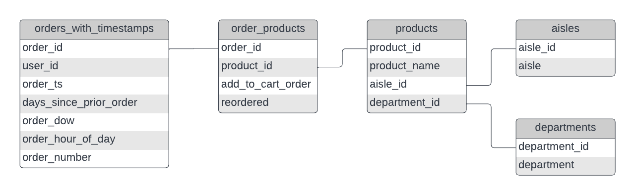
The entity relationship diagram may be helpful and is presented below:
Open BigQuery Console
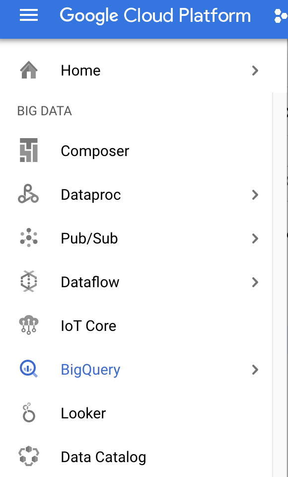
In the Google Cloud Console, select Navigation menu > BigQuery:
The Welcome to BigQuery in the Cloud Console message box opens. This message box provides a link to the quickstart guide and the release notes.
Click Done.
The BigQuery console opens.
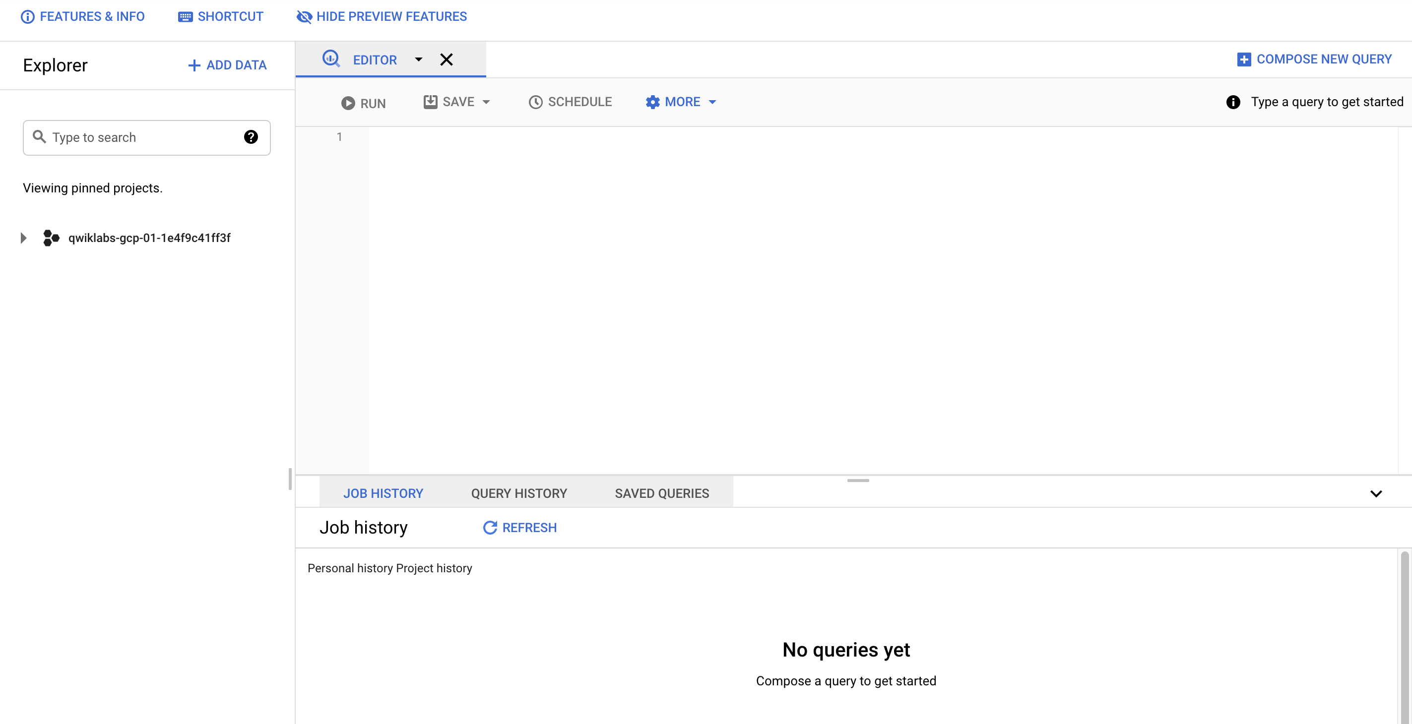
Click on + Compose new query.
Use this query to answer the question:
Note that the bytes billed was approximately 53 MB.
Use this query to answer the question:
The bytes billed was approximately 550 MB.
Use this query to answer the question:
The bytes billed was approximately 745 MB.
Use this query to answer the question:
The bytes billed was approximately 10 MB.
Task 3: Reduce the cost by making use of partitioning
In this task, you will learn to optimize the cost measured in bytes billed for a query by partitioning a table. A partitioned table is divided into segments, called partitions, that make it easier to manage and query your data. By dividing a large table into smaller partitions, you can improve query performance and control costs by reducing the number of bytes read by a query. You partition tables by specifying a partition column which is used to segment the table.
If a query uses a qualifying filter on the value of the partitioning column, BigQuery can scan the partitions that match the filter and skip the remaining partitions. This process is called pruning.
Challenge A : Write a query to find which hour was the busiest in terms of order volume on August 1, 2022.
Original query
Your boss has written a query to solve this challenge.
-
In the SQL Workspace toolbar, click the + Compose new query icon to open the SQL code editor.
-
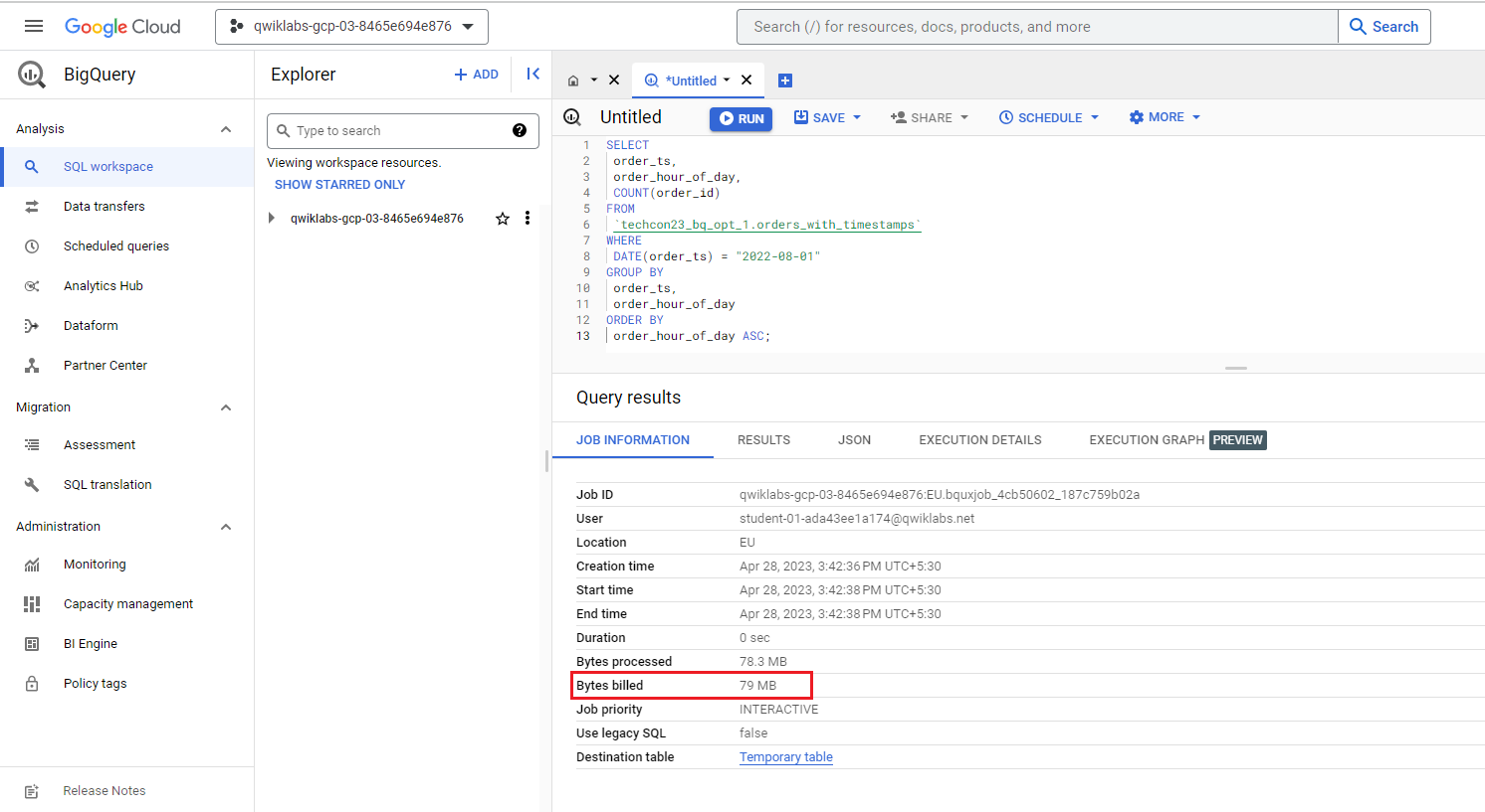
Copy and paste the following query into the BigQuery editor, then click Run.
This query outputs the busiest hour in terms of order volume for 1st August 2022.
Job information details
Your boss noted that the cost of this query, measured in bytes billed, was 79 MB.
- In the Query results pane, under the job information tab, note the number of the bytes billed.
Your boss is unhappy with this query and has asked you to review its performance and optimize it.
Optimize this query using the techniques that you have learned.
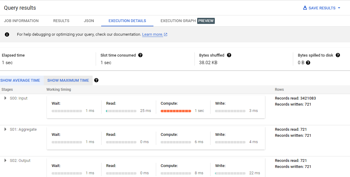
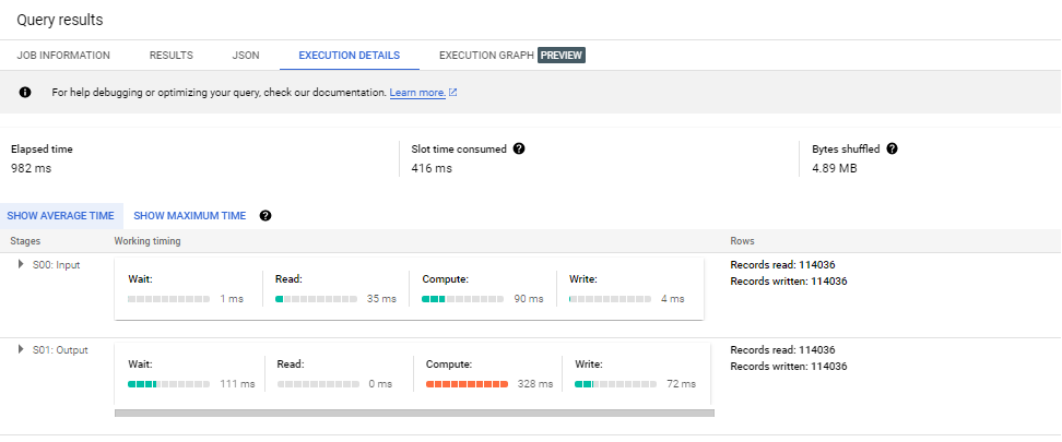
Execution Details
- In the Query results pane, examine the details in the execution details tab.
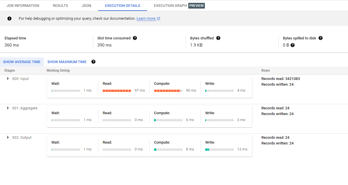
One observation is in stage "S00: Input" you are doing a full table scan, "Records read: 3421083" equals the total number of rows in cymbal_bq_opt_1.orders_with_timestamps. For each record in this table, BigQuery slots are doing Compute to convert a Timestamp to a DATE and compare that to the value "2022-08-01". This is done 3.4 million times.
One way to avoid a full table scan, and to reduce the cost of the query, is to make use of table partitioning.
Optimise the query using table partitioning
- In the BigQuery editor, copy and paste the following query and click the Run button to create a new partitioned table.
Check partioned table creation
- Run a query on this partitioned table to calculate the total order volume by date and hour:
Comparison
As shown in the table below, partitioning greatly reduces bytes billed. This is driven by a massive reduction in records read in stage "S00: Input", achieved by avoiding a full table scan.
| Challenge A (Before) | Challenge A (After) | Improvement | |
|---|---|---|---|
| Bytes billed | 79 MB | 10 MB | 87% reduction |
| No of records read in "S00: Input" | 3,421,083 | 114,036 | 96% reduction |
Task 4: Optimize a query by using denormalization
Challenge B : Your boss has written the following query to find the most popular product sold on August 1, 2022.
- In the BigQuery editor, copy and paste the following query, then click Run:
This query outputs the most popular product sold on August 1, 2022.
Job information details
- In the Query Results pane, under the job information tab, note the number of bytes billed.
Your boss sees that the cost of this query, measured in bytes billed, was 550 MB.
Your boss is unhappy with this query and has asked you to review its performance and optimize it.
Optimize this query using the techniques that you have learned.
Execution details
- In the Query results pane, examine the details in the execution details tab.
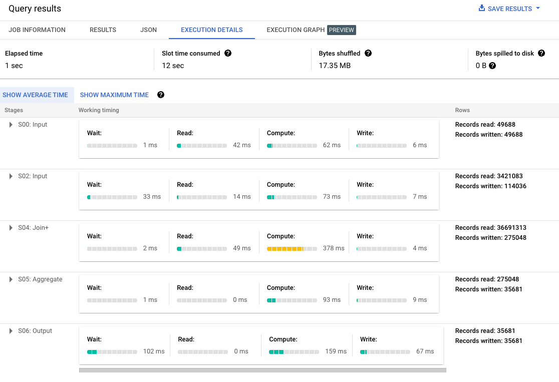
From the job information page, you see that the bytes billed is 550 MB.
One observation is that the most expensive stage is "S03: Join+" as slots are spending time on Compute to join the three input tables. The dataset seems to be in a normalized form. There is a many-to-many relationship between orders and products. One order has many products, and one product may be purchased across many orders. To deal with this, a bridging table called order_products is introduced. This way, there is a 1-to-many relationship on either side of the bridging table. One order has many order_products and one product has many order_products. Because of this normalized structure, three tables need to be joined. This join is very expensive.
For this analytics use case, this normalized Online Transaction Processing (OLTP) approach is not necessary. By de-normalzining the structure of the dataset, you can greatly improve analytical queries.
Optimize the query using denormalization
- Run the following query to achieve this denormalization by using nested and repeated fields:
Check denormalized table creation
- With the new denormalized table created, a query can be written using the following code. Note the query makes use of this technique for flatten arrays.
Comparison
As per the table below, denormalization has a big impact on the cost of the query (measured in bytes billed). This is because, through denormalization, you avoid the three table join that was seen in the original query.
| Challenge B (Before) | Challenge 2B (After) | Improvement | |
|---|---|---|---|
| Bytes billed | 550 MB | 29 MB | 94% reduction |
Task 5: Improve row filtering and join performance by using clustering
Clustered tables in BigQuery are tables that have a user-defined column sort order using clustered columns. Clustered tables can improve query performance and reduce query costs.
In BigQuery, a clustered column is a user-defined table property that sorts storage blocks based on the values in the clustered columns. The storage blocks are adaptively sized based on the size of the table. A clustered table maintains the sort properties in the context of each operation that modifies it. Queries that filter or aggregate by the clustered columns only scan the relevant blocks based on the clustered columns instead of the entire table or table partition. As a result, BigQuery might not be able to accurately estimate the bytes to be processed by the query or the query costs, but it attempts to reduce the total bytes at execution.
Challenge C : The Fraud Team has developed a new ML model, and one of its inputs is the number of products per order. The ML model has predicted that order 1564244 is suspicious. Write a query to report which products were purchased in that order. Report on the sequence in which they were added to the basket.
Write a query to find which product was added to the basket first in this suspicious order.
Original query
- In the BigQuery editor, copy and paste the following query and click Run:
This query finds which product was added to the basket first in this suspicious order.
Job information details
The Fraud Team noticed that the cost of this query, measured in bytes billed, was 497 MB. They are unhappy with this query and have asked you to review its performance and optimize it.
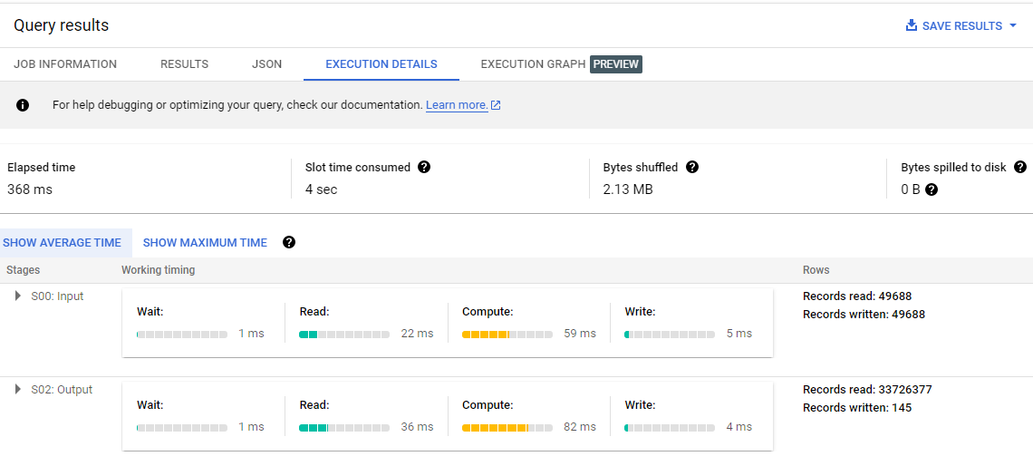
Execution details
- In the query results pane, examine the details in the execution details tab.
Optimize this query using the techniques that you have learned.
To test your skills! Don't peek at the hints until you've had try!
From the job information page, ypu see that the bytes billed is 497 MB.
Examine the execution details tab to see how this could be reduced:
- Stage "S00: Input" is simply loading all 49K rows from
<project_id>.cymbal_bq_opt_1.products. - Stage "S02: Output" is doing two things: scanning all 32 M rows of
<project_id>.cymbal_bq_opt_1. -
order_productsto compare each row's order id with input 1564244 Joining rows from #1 withproject_id. -
cymbal_bq_opt_1.productsonproduct_id.
Clustering of column order_id can help to optimize Stage "S02: Output" as it'll sort the rows in the table and make it easier to look up the rows with order_id = 1564244.
Clustering of column product_id can help optimize this stage as well by improving join performance.
Optimize the query using clustering of column
- In the BigQuery editor, run the following query to cluster by
order_id.
Check cluster by order_id creation
- Run the following query to cluster by
product_id.
Check cluster by product_id creation
- Run the query on these clustered tables to get the desired query result.
Comparison
As shown in the table below, using clustering greatly reduces bytes billed.
| Challenge C (Before) | Challenge 2C (After) | Improvement | |
|---|---|---|---|
| Bytes billed | 497 MB | 20 MB | 95% reduction |
Task 6: Improve dashboard loading speed and cost by using materialized view
In this task you will create materialized view. In BigQuery, materialized views are precomputed views that periodically cache the results of a query for increased performance and efficiency. BigQuery leverages precomputed results from materialized views and whenever possible reads only delta changes from the base tables to compute up-to-date results. Materialized views can be queried directly or can be used by the BigQuery optimizer to process queries to the base tables.
Challenge D : It's the end of the month and your boss wants a chart showing order volume by date and hour for August. Write a SQL query to calculate the total order volume by date and hour. On which date and hour was the most number of orders in August (e.g., 2022-08-11 13H)?
Original query
Your boss was really happy with your hourly order volume table. She discovered, using her amazing BigQuery skills, that this was the query you wrote to create this table.
She was so happy that she added your query to her dashboard. She made a time series chart of hourly sales in August, powered by your query and shared the dashboard with the CEO!
Excited by the email from your boss, the CEO tries to open the dashboard. He is furious; it is very slow to load. The CEO vents his anger by replying to your boss' email. Unfortunately, your boss has just gone on vacation. Her out-of-office auto reply mentions you as point-of-contact for the dashboard. To make matters worse, you do not have edit access to the dashboard, so you cannot edit the query!
Make the query run faster for the CEO and improve dashboard loading speed and cost.
The original loading speed, measured in query Elapsed Time, was around 1,000 ms. What is your new and improved speed?
The original cost, measured in bytes billed, was around 27MB. What is your new and reduced cost?
The answer here is to use a materialized view.
In particular you need to use smart-tuning to make the hidden read-only query in the dashboard use of your new materialized view.
Execution details
- In the Query results pane, examine the details in the execution details tab.
As per stage "S00: Input" you're doing a full table scan of cymbal_bq_opt_1.orders_with_timestamps which is likely the reason for the slow performance and high cost.
You need to create a materialized view with the same logic in the same dataset cymbal_bq_opt_1 .
Optimize the query using materialized view and smart tuning
- In the BigQuery editor, run the following query to create a materialized view:
Check materialized view creation
- Run the original query again, now smart-rewritten by materialized view, to get the desired query result:
Execution details after using materialized views
- In the Query results pane, examine the details in the execution details tab.
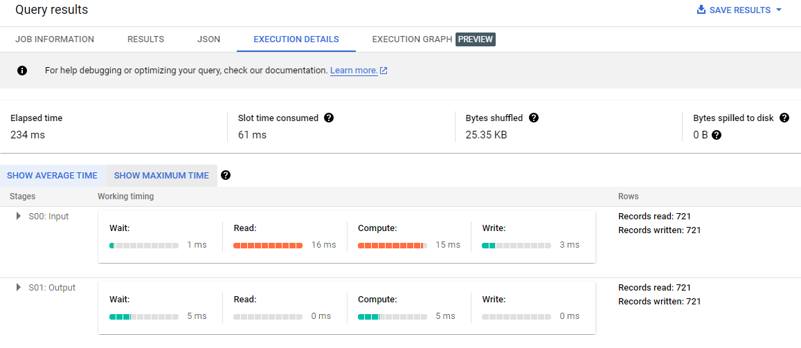
As per stage "S00: Input", you are no longer reading from the base table, but are now reading from the materialized view (via the "smart tuning" feature).
Comparison
The overall impact of using a materialized view is that costs are reduced and query speed improves.
| Challenge D (Before) | Challenge D (After) | Improvement | |
|---|---|---|---|
| Bytes billed | 27 MB | 10 MB | 62% reduction |
| Elapsed Time | 1,000 ms | 389 ms | 61% reduction |
The CEO is impressed and your boss gives you a raise!
Task 7: Reduce the elapsed time and cost by pruning partition with a filter
Challenge E : Your boss has asked for a report for the order IDs on the day with the most customers. Your colleague has written the following SQL to pull the report.
Original query
- In the BigQuery editor, copy and paste the following query and click Run.
Your boss has told your colleague that the query is too expensive, with bytes billed = 79 MB.
As the resident BigQuery expert, your colleague comes to you for help and advice to reduce this cost.
The original cost, measured in bytes billed, was around 79MB. What is your new and reduced cost?
Execution details
- In the Query results pane, examine the execution details of the original query.
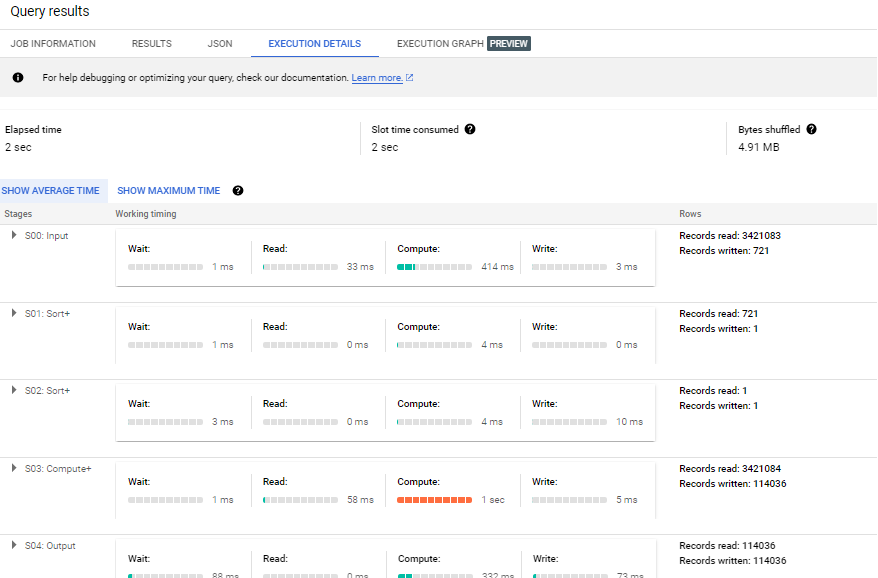
The Execution Details page shows that you are doing a full table scan. Stage "S00: Input" is reading all 3.4 million rows of the table. To help avoid this, partition the table.
Optimize the query using partitioning
- Run the below query in the BigQuery editor to partition the table by date(order_ts):
Check table partition by order_ts creation
- Run the query against against the newly partition table:
Execution details after partitioning
- In the query results pane, revisit the execution details page now.
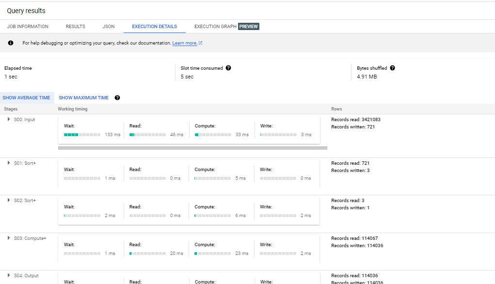
The Execution Details page shows that you are still doing a full table scan. The subquery is not pruning partitions, but the query is executing faster than before (from 2 sec to 1 sec). The number of bytes billed is not reduced from the original query (seen in the Job Information tab).
Optimize by pruning partition with a filter
By inspecting the results table of query 2, the target date was found to be "2022-08-17". What happens if you do not write a subquery and instead just provide this date directly as per the query below:
Execution details after pruning partition with a filter
- In the Query results pane, revisit the execution details page now.
Now you are no longer doing a full table scan. You are making use of the partitioning and pruning the partition with the filter on the provided date string. This is seen in stage "S00: Input" where you are no longer reading the full 3.2M rows of the table. You have again reduced the elapsed time (2 sec reduced to 1 sec). As per the job information page, the bytes billed have been reduced from 79MB to 10MB.
| query | bytes billed | bytes saved | elapsed time | time reduction |
|---|---|---|---|---|
| original query | 79 MB | - | 2 seconds | - |
| query 2 | 79 MB | 0% | 1 second | 50% |
| query 3 | 10 MB | 87% | 1 second | 50% |
As per the table above, adding partitioning alone reduces the elapsed time by 50%, but does not reduce the bytes billed. This is because of the way BigQuery handles pruning of partitions through subqueries. This also occurs when pruning partitions through joins, but they were not explored in this challenge.
For customers using on-demand pricing, this is important to remember. Adding partitioning alone does not reduce the financial costs if a query is using subqueries or joins to prune partitions.
Congratulations
By working through several scenarios you've learned how to reduce the bytes billed by through partitioning and pruning the partiion with filters; optimize a query using denormalization; and improved row filtering and join performance with clustering. You have improved dashboard loading speed and cost by using the materialized view.
Google Cloud Training & Certification
...helps you make the most of Google Cloud technologies. Our classes include technical skills and best practices to help you get up to speed quickly and continue your learning journey. We offer fundamental to advanced level training, with on-demand, live, and virtual options to suit your busy schedule. Certifications help you validate and prove your skill and expertise in Google Cloud technologies.
Manual Last Updated November 01, 2023
Lab Last Tested November 01, 2023
Copyright 2023 Google LLC All rights reserved. Google and the Google logo are trademarks of Google LLC. All other company and product names may be trademarks of the respective companies with which they are associated.